6 Appendix
6.1 More on Dealing with Non-numeric data
So far, we’ve primarily worked with numeric data.
Let’s talk briefly about how R handles string or character data.
Here’s a data frame with some letters.
myname <- data.frame(letter=c("k","e","l","s","e","y"))Let’s look at the structure of the myname object, and the letter field of the object.
myname %>% str()## 'data.frame': 6 obs. of 1 variable:
## $ letter: Factor w/ 5 levels "e","k","l","s",..: 2 1 3 4 1 5myname$letter %>% str()## Factor w/ 5 levels "e","k","l","s",..: 2 1 3 4 1 5Hmm, it says Factor w/ 5 levels "e","k","l","s",..: 2 1 3 4 1 5. What does this mean?
By default, R stores string fields in data frames as factors.
Behind the scenes, R identifies the unique character strings in the field, substitutes each one with a unique integer, and remembers the original strings as levels.
myname$letter %>% levels()## [1] "e" "k" "l" "s" "y"myname$letter %>% as.integer()## [1] 2 1 3 4 1 5For many processes and analyses, this data structure will work fine.
In some situations, however, it becomes problematic.
Let’s try to modify the myname data frame, and make the letters spell out kelseysm rather than kelsey.
We need to add letters s and m to the next rows. We can do that with the rbind function.
myname <- myname %>% rbind("s")
myname <- myname %>% rbind("m")
## Warning in `[<-.factor`(`*tmp*`, ri, value = "m"): invalid factor level, NA
## generatedAn Error! That’s not what we want. This happened because “m” is not a registerd factor for letter, so R won’t add it.
There are a couple of ways to override R’s default behavior of storing text fields as columns.
If we’re creating a data frame from scratch, we can set the stringsAsFactors parameter equal to FALSE.
myname <- data.frame(letter=c("k","e","l","s","e","y"), stringsAsFactors=FALSE)Check out the structure str and see what is different.
Let’s try making the same modifications now.
myname <- myname %>% rbind("s")
myname <- myname %>% rbind("m")
The character data type is much more flexible.
If we’ve already created (or read) a data frame, we can use the as.character function on the text field itself.
myname <- data.frame(letter=c("k","e","l","s","e","y"))
myname %>% str()
## 'data.frame': 6 obs. of 1 variable:
## $ letter: Factor w/ 5 levels "e","k","l","s",..: 2 1 3 4 1 5myname$letter <- myname$letter %>% as.character()
myname %>% str()## 'data.frame': 6 obs. of 1 variable:
## $ letter: chr "k" "e" "l" "s" ...myname <- myname %>% rbind("s")
myname <- myname %>% rbind("m")Looking out for factors is critical when typecasting numeric data that is mistakenly stored as text.
Here’s another data frame.
fives <- data.frame(v1=c("5","10","15","20"))Let’s look at the structure and levels:
fives %>% str()## 'data.frame': 4 obs. of 1 variable:
## $ v1: Factor w/ 4 levels "10","15","20",..: 4 1 2 3fives$v1 %>% levels()## [1] "10" "15" "20" "5"We want these data points stored as a numeric type, but currently, they’re stored as text and, specifically, as a factor.
What does it look like if we convert the factor to numeric?
fives$v1 %>% as.numeric()## [1] 4 1 2 3So problematic! Why did this happen?
Because the factor levels are what is converted to numbers, not the characters inside the strings. Let’s first convert factors to characters and then convert to numbers.
fives$v1 %>% as.character() %>% as.numeric()## [1] 5 10 15 20That works as expected.
Are factors ever useful? Yes.
Here’s some pretend survey data.
survey <- data.frame(gender=rep(c("Male", "Female"), c(5, 7)), response=rep(c("Excellent", "Good", "Fair", "Poor"), 3))Let’s change the levels of the gender field.
survey$gender %>% levels()## [1] "Female" "Male"levels(survey$gender) <- c("F","M")What does it look like now?
We can also take advantage of our understanding of the factor data type to convert the response variable into a numeric field.
I want excellent to map to 4, good to map to 3, fair to map to 2 and poor to map to 1.
We’ll use the as.numeric function eventually, but first we need to see if the levels are in the order that we want them.
survey$response %>% levels()## [1] "Excellent" "Fair" "Good" "Poor"They’re not. Let’s change them, so that less favorable responses will appear before more favorable responses when alphabetized.
After we change the levels, we’ll need to turn the response field into a character field, and then re-factor.
levels(survey$response) <- c("D Excellent","B Fair","C Good","A Poor")
survey$response <- survey$response %>% as.character() %>% as.factor()
survey$response %>% levels()
## [1] "A Poor" "B Fair" "C Good" "D Excellent"levels(survey$response) <- c("Poor","Fair","Good","Excellent")Much better. Now we can call the as.numeric function.
survey %>% mutate(as.numeric(response))## gender response as.numeric(response)
## 1 M Excellent 4
## 2 M Good 3
## 3 M Fair 2
## 4 M Poor 1
## 5 M Excellent 4
## 6 F Good 3
## 7 F Fair 2
## 8 F Poor 1
## 9 F Excellent 4
## 10 F Good 3
## 11 F Fair 2
## 12 F Poor 1How useful!
6.1.1 The takeaway
By default, R stores text fields as factors. And factors are strange.
At times it seems like they are working against us.
But if we understand how they work, we can make them work for us!
Now, back to numeric data.
6.1.2 Controlling order
For the boxplot, if instead of warm and cool, we’d used high and low to bin the temperatures, we would need to use factors to help us put the plots in order.
aircomplete <- aircomplete %>% mutate(Temp2 = ifelse(Temp > 80, "high", "low"))We are using mutate from the dplyr package to add a new column Temp2, which is a character data type based on the variable Temp.
Next, let us create a box plot using this new Temp2 variable. We can use geom_boxplot to create this plot.
ggplot(aircomplete) + geom_boxplot(aes(x=Temp2, y=Ozone))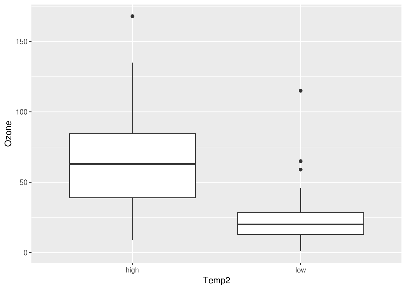
We see that low shows up after high on the x axis, and it is counter-intuitive. This is because Temp2 is a character, which is sorted alphabetically (h before l). So we can use factors, as explained in the previous section, to switch their position.
aircomplete <- aircomplete %>% mutate(Temp_factor = factor(Temp2, levels = c("low", "high")))
aircomplete %>% str()
## 'data.frame': 111 obs. of 8 variables:
## $ Ozone : int 41 36 12 18 23 19 8 16 11 14 ...
## $ Solar.R : int 190 118 149 313 299 99 19 256 290 274 ...
## $ Wind : num 7.4 8 12.6 11.5 8.6 13.8 20.1 9.7 9.2 10.9 ...
## $ Temp : int 67 72 74 62 65 59 61 69 66 68 ...
## $ Month : int 5 5 5 5 5 5 5 5 5 5 ...
## $ Day : int 1 2 3 4 7 8 9 12 13 14 ...
## $ Temp2 : chr "low" "low" "low" "low" ...
## $ Temp_factor: Factor w/ 2 levels "low","high": 1 1 1 1 1 1 1 1 1 1 ...Again, we use mutate to add another new column Temp_factor, which is a factor version of Temp2. Also, you will notice we have explicitly specified the levels in an order we would like (low and then high). This is confirmed in the str command.
Alright! Now let’s see how Temp_factor looks in our boxplot.
ggplot(aircomplete) + geom_boxplot(aes(x=Temp_factor, y=Ozone))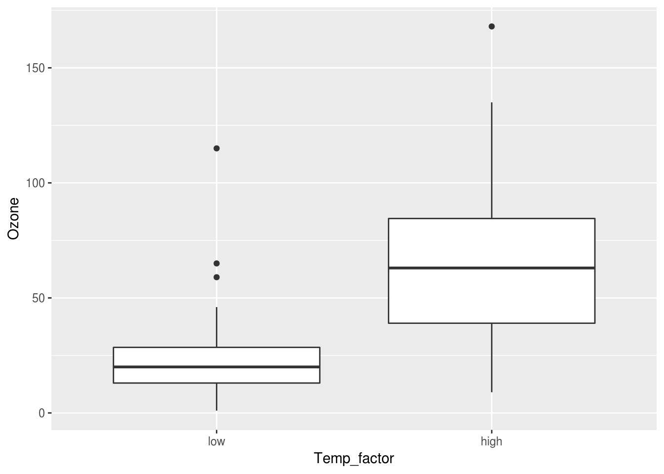
6.2 Webscraping and text analysis
6.3 Machine Learning in R
6.4 Interactive R Graphics
- Interactive visualizations with R
- “A minireview of R packages ggvis, rCharts, plotly and googleVis for interactive visualizations”
- Shiny Tutorial
- Plotly ggplot
- Flex Dashboard
6.5 Maps
- Leaflet for R
- Intro to making interactive maps in R
- Spatial Data with R
- Making Maps with R
- R-Bloggers search for maps